Analyzing Supernova Data
Overview
Teaching: 30 min
Exercises: 10 minQuestions
How can I process tabular data files in Python?
Objectives
Explain what a library is and what libraries are used for.
Import a Python library and use the functions it contains.
Read tabular data from a file into a program.
Assign values to variables.
Select individual values and subsections from data.
Perform operations on arrays of data.
Plot simple graphs from data.
In this episode we will learn how to work with supenovae lightcurve data in Python. However, before we discuss how to deal with many data points, let’s learn how to work with single data values.
Variables
Any Python interpreter can be used as a calculator:
3 + 5 * 4
23
This is great but not very interesting.
To do anything useful with data, we need to assign its value to a variable.
In Python, we can assign a value to a
variable, using the equals sign =.
For example, to assign value 60 to a variable weight_kg, we would execute:
weight_kg = 60
From now on, whenever we use weight_kg, Python will substitute the value we assigned to
it. In essence, a variable is just a name for a value.
In Python, variable names:
- can include letters, digits, and underscores
- cannot start with a digit
- are case sensitive.
This means that, for example:
weight0is a valid variable name, whereas0weightis notweightandWeightare different variables
Types of data
Python knows various types of data. Three common ones are:
- integer numbers
- floating point numbers, and
- strings.
In the example above, variable weight_kg has an integer value of 60.
To create a variable with a floating point value, we can execute:
weight_kg = 60.0
And to create a string we simply have to add single or double quotes around some text, for example:
weight_kg_text = 'weight in kilograms:'
Using Variables in Python
To display the value of a variable to the screen in Python, we can use the print function:
print(weight_kg)
60.0
We can display multiple things at once using only one print command:
print(weight_kg_text, weight_kg)
weight in kilograms: 60.0
Moreover, we can do arithmetics with variables right inside the print function:
print('weight in pounds:', 2.2 * weight_kg)
weight in pounds: 132.0
The above command, however, did not change the value of weight_kg:
print(weight_kg)
60.0
To change the value of the weight_kg variable, we have to
assign weight_kg a new value using the equals = sign:
weight_kg = 65.0
print('weight in kilograms is now:', weight_kg)
weight in kilograms is now: 65.0
Variables as Sticky Notes
A variable is analogous to a sticky note with a name written on it: assigning a value to a variable is like putting that sticky note on a particular value.
This means that assigning a value to one variable does not change values of other variables. For example, let’s store the subject’s weight in pounds in its own variable:
# There are 2.2 pounds per kilogram
weight_lb = 2.2 * weight_kg
print(weight_kg_text, weight_kg, 'and in pounds:', weight_lb)
weight in kilograms: 65.0 and in pounds: 143.0
Let’s now change
weight_kg:weight_kg = 100.0 print('weight in kilograms is now:', weight_kg, 'and weight in pounds is still:', weight_lb)weight in kilograms is now: 100.0 and weight in pounds is still: 143.0
Since
weight_lbdoesn’t “remember” where its value comes from, it is not updated when we changeweight_kg.


Words are useful, but what’s more useful are the sentences and stories we build with them. Similarly, while a lot of powerful, general tools are built into Python, specialized tools built up from these basic units live in libraries that can be called upon when needed.
Loading data into Python
In order to load our supernova data, we need to access (import in Python terminology) a library called NumPy. In general you should use this library if you want to do fancy things with numbers, especially if you have matrices or arrays. We can import NumPy using:
import numpy
Importing a library is like getting a piece of lab equipment out of a storage locker and setting it up on the bench. Libraries provide additional functionality to the basic Python package, much like a new piece of equipment adds functionality to a lab space. Just like in the lab, importing too many libraries can sometimes complicate and slow down your programs - so we only import what we need for each program. Once we’ve imported the library, we can ask the library to read our data file for us:
numpy.loadtxt(fname='data/03D1ar.csv', delimiter=',', skiprows=1)
array([[ 5.28805e+04,  1.30350e+01,  5.42460e+00,          nan,
                 nan,          nan,          nan,          nan,
                 nan],
       [ 5.28815e+04,          nan,          nan,  7.02820e+00,
         9.91050e+00,  1.61570e+01,  1.86290e+01,  2.20860e+01,
         7.19510e+01],
         ...,
       [ 5.30262e+04,          nan,          nan,          nan,
                 nan,  5.10690e+01,  2.02770e+01,          nan,
                 nan],
       [ 5.30263e+04,          nan,          nan,  6.58160e+00,
         1.16650e+01,          nan,          nan,          nan,
                 nan]])
The expression numpy.loadtxt(...) is a function call
that asks Python to run the function loadtxt which
belongs to the numpy library. This dotted notation
is used everywhere in Python: the thing that appears before the dot contains the thing that
appears after.
As an example, John Smith is the John that belongs to the Smith family.
We could use the dot notation to write his name smith.john,
just as loadtxt is a function that belongs to the numpy library.
numpy.loadtxt has three parameters: the name of the file
we want to read, the delimiter that separates values on
a line and a statement to skip the first row. The first two need to be character strings
(or strings
for short), so we put them in quotes. The last one is an integer and we do not use quotes.
Since we haven’t told it to do anything else with the function’s output,
the terminal/notebook displays it.
In this case,
that output is the data we just loaded.
By default,
only a few rows and columns are shown
(with ... to omit elements when displaying big arrays).
To save space,
Python displays numbers as 1. instead of 1.0
when there’s nothing interesting after the decimal point.
Our call to numpy.loadtxt read our file
but didn’t save the data in memory.
To do that,
we need to assign the array to a variable. Just as we can assign a single value to a variable, we
can also assign an array of values to a variable using the same syntax. Let’s re-run
numpy.loadtxt and save the returned data:
data = numpy.loadtxt(fname='data/03D1a1.csv', delimiter=',', skiprows=1)
This statement doesn’t produce any output because we’ve assigned the output to the variable data.
If we want to check that the data have been loaded,
we can print the variable’s value:
print(data)
       ([[ 5.28805e+04,  1.30350e+01,  5.42460e+00,          nan,
                 nan,          nan,          nan,          nan,
                 nan],
       [ 5.28815e+04,          nan,          nan,  7.02820e+00,
         9.91050e+00,  1.61570e+01,  1.86290e+01,  2.20860e+01,
         7.19510e+01],
         ...,
       [ 5.30262e+04,          nan,          nan,          nan,
                 nan,  5.10690e+01,  2.02770e+01,          nan,
                 nan],
       [ 5.30263e+04,          nan,          nan,  6.58160e+00,
         1.16650e+01,          nan,          nan,          nan,
                 nan]])
Now that the data are in memory,
we can manipulate them.
First,
let’s ask what type of thing data refers to:
print(type(data))
<class 'numpy.ndarray'>
The output tells us that data currently refers to
an N-dimensional array, the functionality for which is provided by the NumPy library.
These data correspond to the fluxes of a supernova as a function of time.
The rows are the days of the observations, and the columns
the brightness measurements.
Data Type
A Numpy array contains one or more elements of the same type. The
typefunction will only tell you that a variable is a NumPy array but won’t tell you the type of thing inside the array. We can find out the type of the data contained in the NumPy array.print(data.dtype)dtype('float64')This tells us that the NumPy array’s elements are floating-point numbers.
With the following command, we can see the array’s shape:
print(data.shape)
(48, 9)
The output tells us that the data array variable contains 48 rows and 9 columns. When we
created the variable data to store our data, we didn’t just create the array; we also
created information about the array, called members or
attributes. This extra information describes data in the same way an adjective describes a noun.
data.shape is an attribute of data which describes the dimensions of data. We use the same
dotted notation for the attributes of variables that we use for the functions in libraries because
they have the same part-and-whole relationship.
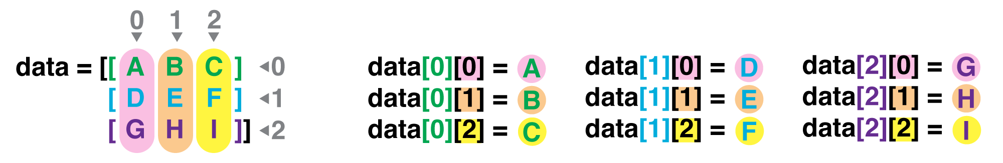
If we want to get a single number from the array, we must provide an index in square brackets after the variable name, just as we do in math when referring to an element of a matrix. Our supernova data has two dimensions, so we will need to use two indices to refer to one specific value:
print('first value in data:', data[0, 0])
first value in data: 52880.5
print('middle value in data:', data[24,5])
middle value in data: 162.78
The expression data[24,5] accesses the element at row 24, column 5. While this expression may
not surprise you,
data[0, 0] might.
Programming languages like Fortran, MATLAB and R start counting at 1
because that’s what human beings have done for thousands of years.
Languages in the C family (including C++, Java, Perl, and Python) count from 0
because it represents an offset from the first value in the array (the second
value is offset by one index from the first value). This is closer to the way
that computers represent arrays (if you are interested in the historical
reasons behind counting indices from zero, you can read
Mike Hoye’s blog post).
As a result,
if we have an M×N array in Python,
its indices go from 0 to M-1 on the first axis
and 0 to N-1 on the second.
It takes a bit of getting used to,
but one way to remember the rule is that
the index is how many steps we have to take from the start to get the item we want.
In the Corner
What may also surprise you is that when Python displays an array, it shows the element with index
[0, 0]in the upper left corner rather than the lower left. This is consistent with the way mathematicians draw matrices but different from the Cartesian coordinates. The indices are (row, column) instead of (column, row) for the same reason, which can be confusing when plotting data.
Slicing data
An index like [24,5] selects a single element of an array,
but we can select whole sections as well.
For example,
we can select the first ten days (columns) of values
for the first four patients (rows) like this:
print(data[0:4, 0:9])
[[5.28805e+04, 1.30350e+01, 5.42460e+00,         nan,         nan,
                nan,         nan,         nan,         nan],
       [5.28815e+04,         nan,         nan, 7.02820e+00, 9.91050e+00,
        1.61570e+01, 1.86290e+01, 2.20860e+01, 7.19510e+01],
       [5.28866e+04,         nan,         nan,         nan,         nan,
        1.89440e+02, 1.98550e+01,         nan,         nan],
       [5.29005e+04, 1.42800e+02, 1.49700e+01, 4.57050e+02, 1.69190e+01,
        6.54020e+02, 2.32020e+01, 5.72040e+02, 8.95940e+01]]
The slice 0:4 means, “Start at index 0 and go up to, but not
including, index 4.”Again, the up-to-but-not-including takes a bit of getting used to, but the
rule is that the difference between the upper and lower bounds is the number of values in the slice.
We don’t have to start slices at 0:
print(data[5:10, 0:9])
[[5.29046e+04, 1.14730e+02, 7.55460e+00,         nan,         nan,
                nan,         nan,         nan,         nan],
       [5.29085e+04, 8.49230e+01, 7.51630e+00, 3.84570e+02, 1.27970e+01,
                nan,         nan,         nan,         nan],
       [5.29086e+04,         nan,         nan,         nan,         nan,
        6.04660e+02, 2.04640e+01,         nan,         nan],
       [5.29096e+04,         nan,         nan,         nan,         nan,
                nan,         nan, 6.69740e+02, 8.09650e+01],
       [5.29124e+04,         nan,         nan,         nan,         nan,
        5.70830e+02, 1.95730e+01,         nan,         nan]]
We also don’t have to include the upper and lower bound on the slice. If we don’t include the lower bound, Python uses 0 by default; if we don’t include the upper, the slice runs to the end of the axis, and if we don’t include either (i.e., if we just use ‘:’ on its own), the slice includes everything:
small = data[:3, 7:]
print('small is:')
print(small)
The above example selects rows 0 through 2 and columns 7 through to the end of the array.
small is:
[[   nan,    nan],
 [22.086, 71.951],
 [   nan,    nan]]
Arrays also know how to perform common mathematical operations on their values. The simplest operations with data are arithmetic: addition, subtraction, multiplication, and division. When you do such operations on arrays, the operation is done element-by-element. Thus:
doubledata = data * 2.0
will create a new array doubledata
each element of which is twice the value of the corresponding element in data:
print('original:')
print(data[:3, 7:])
print('doubledata:')
print(doubledata[:3, 7:])
original:
[[   nan,    nan],
 [22.086, 71.951],
 [   nan,    nan]]
doubledata:
[[    nan,     nan],
 [ 44.172, 143.902],
 [    nan,     nan]]
If, instead of taking an array and doing arithmetic with a single value (as above), you did the arithmetic operation with another array of the same shape, the operation will be done on corresponding elements of the two arrays. Thus:
tripledata = doubledata + data
will give you an array where tripledata[0,0] will equal doubledata[0,0] plus data[0,0],
and so on for all other elements of the arrays.
print('tripledata:')
print(tripledata[:3, 7:])
tripledata:
[[    nan,     nan],
 [ 66.258, 215.853],
 [    nan,     nan]]
Often, we want to do more than add, subtract, multiply, and divide array elements. NumPy knows how
to do more complex operations, too. If we want to find the average for the g band on, for example,
we can ask NumPy to compute data’s mean value:
print(numpy.mean(data[:,1])))
nan
mean is a function that takes
an array as an argument. In this case we
have a lot of NaNs in the column and mean cannot calculate a proper value.
A sister function, nanmean, can ignore the NaNs:
print(numpy.nanmean(data[:,1])))
27.096660000000004
Not All Functions Have Input
Generally, a function uses inputs to produce outputs. However, some functions produce outputs without needing any input. For example, checking the current time doesn’t require any input.
import time
print(time.ctime())
'Sat Mar 26 13:07:33 2016'For functions that don’t take in any arguments, we still need parentheses (
()) to tell Python to go and do something for us.
NumPy has lots of useful functions that take an array as input. Let’s use three of those functions to get some descriptive values about the dataset. We’ll also use multiple assignment, a convenient Python feature that will enable us to do this all in one line.
maxval, minval, stdval = numpy.nanmax(data[:,1]), numpy.nanmin(data[:,1]), numpy.nanstd(data[:,1])

print('maximum flux:', maxval)
print('minimum flux:', minval)
print('standard deviation:', stdval)
Here we’ve assigned the return value from numpy.max(data) to the variable maxval, the value
from numpy.min(data) to minval, and so on.
maximum flux: 142.8
minimum flux: -28.9
standard deviation: 53.4821178405979
Mystery Functions in IPython
How did we know what functions NumPy has and how to use them? If you are working in IPython or in a Jupyter Notebook, there is an easy way to find out. If you type the name of something followed by a dot, then you can use tab completion (e.g. type
numpy.and then press tab) to see a list of all functions and attributes that you can use. After selecting one, you can also add a question mark (e.g.numpy.cumprod?), and IPython will return an explanation of the method! This is the same as doinghelp(numpy.cumprod).
When analyzing data, though, we often want to look at variations in statistical values, such as the maximum brightness per band or object or the average brightness per band. One way to do this is to create a new temporary array of the data we want, then ask it to do the calculation:
Flux_r = data[:, 3] # everything on the first axis (rows), the fourth on the second axis (columns)
print('maximum flux in g band is:', numpy.nanmax(Flux_r))
maximum flux in g band is: 457.05
Everything in a line of code following the ‘#’ symbol is a comment that is ignored by Python. Comments allow programmers to leave explanatory notes for other programmers or their future selves.
We don’t actually need to store the column in a variable of its own. Instead, we can combine the selection and the function call:
print('maximum flux in i band is:', np.nanmax(data[:,5]))
maximum flux in i band is: 694.11
What if we need the maximum flux for each day in any band (as in the next diagram on the left) or the average for band (as in the diagram on the right)? As the diagram below shows, we want to perform the operation across an axis:
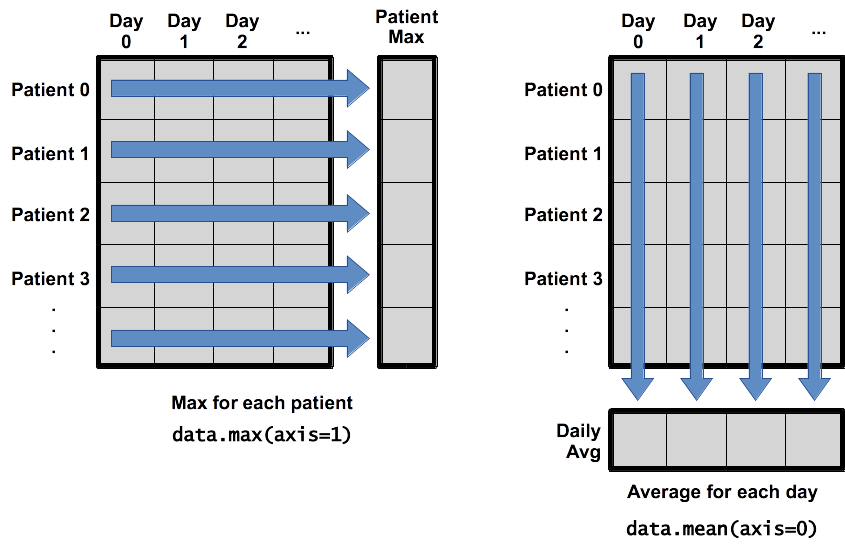
To support this functionality, most array functions allow us to specify the axis we want to work on. If we ask for the average across axis 0 (rows in our 2D example), we get:
print(numpy.nanmean(data, axis=0))
[5.29537333e+04 2.70966600e+01 8.93325833e+00 8.81428870e+01
 1.79726304e+01 2.19487541e+02 2.21493182e+01 2.12659100e+02
 8.72582000e+01]
As a quick check, we can ask this array what its shape is:
print(numpy.nanmean(data, axis=0).shape)
(9,)
The expression (9,) tells us we have an N×1 vector,
so this is the average value for each column.
If we average across axis 1 (columns in our 2D example), we get:
print(numpy.nanmean(data, axis=1))
[ 9.22980000e+00  2.42936167e+01  1.04647500e+02  2.46324375e+02
  2.81024250e+02  6.11423000e+01  1.22451575e+02  3.12562000e+02
  3.75352500e+02  2.95201500e+02  1.15507000e+02  2.65575000e+02
  1.41784500e+02  1.53148000e+02  2.02829000e+01  2.11857250e+01
  1.24418500e+02  1.40559500e+02  1.84695000e+01  2.03128000e+01
  1.03193500e+02  2.19719500e+01  2.74837500e+02  8.96285000e+01
  4.87550300e+01  6.33962500e+01  4.06410000e+01  1.69725000e-01
  9.37185000e+01  3.22807750e+01  6.46100000e+01  4.53500000e-01
  8.37650000e+01  4.63065000e+01  3.75445000e+00  2.00239000e+01
 -1.00273500e+01  2.33642500e+01  9.52407500e+00  3.14025000e-01
  5.06840000e+01  3.12785000e+01  1.50105000e+01  2.13955000e+01
  3.79590000e+01  1.18775000e+01  3.56730000e+01  9.12330000e+00]
which is the average flux for each day of observations.
Other Fun Numpy Features
A common task in working with arrays is to subselect all elements that satisfy a condition . In IDL this task is
carried out by the where function which returns the indexes of the array elements that satisfy the condition which the user can then iterrate over. While
there is a numpy.where task, Python allows
for a more elegant execution of this workflow. Python allows for a direct comparison between a numpy array and a float or integer which returns a Boolean array.
index = data[:,1] > 100
print(index)
[False False False  True False  True False False False False False False
 False False False False False False False False False False False False
 False False False False False False False False False False False False
 False False False False False False False False False False False False]
In arithmetic operations with Boolean arrays, the values True and False are interpreted as 1 and 0respectively. One easy way to find out how many items satisfied the condition (i.e. how many True values there are in the index array) is to sum the index array:
numpy.sum(index)
2
This Boolean array can then be used as an index:
print(data[:,1][index])
print(data[:,1][index]+200.)
print(data[:,0][index])
[142.8  114.73]
[242.8  214.73]
[52900.5 52904.6]
Numpy allow for the creating of empty arrays of several different types. For example to create an array of zeros:
numpy.zeros(5)
array([0., 0., 0., 0., 0.])
By default the data type is float. Try the following two examples:
numpy.zeros(5, dtype=int)
numpy.zeros(5, dtype=bool)
Similar to numpy.zero are numpy.one which creates an array of ones, numpy.fill which creates an array filled with a specified value and numpy.empy which creats an “empty” array. On one hand numpy.empty does not set the array values to zero, and may therefore be marginally faster. On the other hand, it requires the user to manually set all the values in the array, and should be used with caution.
A final numpy trick is to check if a value is NaN or to find where all the NaNs are withing an array:
np.isnan(data[:,1])
The output is again a Boolean array.
Scientists Dislike Typing
We will always use the syntax
import numpyto import NumPy. However, in order to save typing, it is often suggested to make a shortcut like so:import numpy as np. If you ever see Python code online using a NumPy function withnp(for example,np.loadtxt(...)), it’s because they’ve used this shortcut. When working with other people, it is important to agree on a convention of how common libraries are imported.
Check Your Understanding
What values do the variables
massandagehave after each statement in the following program? Test your answers by executing the commands.mass = 47.5 age = 122 mass = mass * 2.0 age = age - 20 print(mass, age)Solution
95.0 102
Sorting Out References
What does the following program print out?
first, second = 'Grace', 'Hopper'
third, fourth = second, first
print(third, fourth)
Solution
Hopper Grace
Slicing Strings
A section of an array is called a slice. We can take slices of character strings as well:
element = 'oxygen'
print('first three characters:', element[0:3])
print('last three characters:', element[3:6])
first three characters: oxy last three characters: genWhat is the value of
element[:4]? What aboutelement[4:]? Orelement[:]?Solution
oxyg
en
oxygen
What is
element[-1]? What iselement[-2]?Solution
n
e
Given those answers, explain what
element[1:-1]does.Solution
Creates a substring from index 1 up to (not including) the final index, effectively removing the first and last letters from ‘oxygen’
Thin Slices
The expression
element[3:3]produces an empty string, i.e., a string that contains no characters. Ifdataholds our array of patient data, what doesdata[3:3, 4:4]produce? What aboutdata[3:3, :]?Solution
[]
[]
Plot Scaling
Why do all of our plots stop just short of the upper end of our graph?
Solution
Because matplotlib normally sets x and y axes limits to the min and max of our data (depending on data range)
If we want to change this, we can use the
set_ylim(min, max)method of each ‘axes’, for example:axes3.set_ylim(0,6)Update your plotting code to automatically set a more appropriate scale. (Hint: you can make use of the
maxandminmethods to help.)Solution
# One method
axes3.set_ylabel('min')
axes3.plot(numpy.min(data, axis=0))
axes3.set_ylim(0,6)
Solution
# A more automated approach
min_data = numpy.min(data, axis=0)
axes3.set_ylabel('min')
axes3.plot(min_data)
axes3.set_ylim(numpy.min(min_data), numpy.max(min_data) * 1.1)
Make Your Own Plot
Create a plot showing the standard deviation (
numpy.std) of the flux for each day of observations.Solution
std_plot = matplotlib.pyplot.plot(numpy.nanstd(data[:,1:], axis=0))
matplotlib.pyplot.show()
Moving Plots Around (DO NOT USE)
Modify the program to display the three plots on top of one another instead of side by side.
Solution
import numpy
import matplotlib.pyplot

data = numpy.loadtxt(fname='data/03D1ar.csv', delimiter=',')

# change figsize (swap width and height)
fig = matplotlib.pyplot.figure(figsize=(3.0, 10.0))

# change add_subplot (swap first two parameters)
axes1 = fig.add_subplot(3, 1, 1)
axes2 = fig.add_subplot(3, 1, 2)
axes3 = fig.add_subplot(3, 1, 3)

axes1.set_ylabel('average')
axes1.plot(numpy.mean(data, axis=0))

axes2.set_ylabel('max')
axes2.plot(numpy.max(data, axis=0))

axes3.set_ylabel('min')
axes3.plot(numpy.min(data, axis=0))

fig.tight_layout()

matplotlib.pyplot.show()
Stacking Arrays
Arrays can be concatenated and stacked on top of one another, using NumPy’s
vstackandhstackfunctions for vertical and horizontal stacking, respectively.import numpy A = numpy.array([[1,2,3], [4,5,6], [7, 8, 9]]) print('A = ') print(A) B = numpy.hstack([A, A]) print('B = ') print(B) C = numpy.vstack([A, A]) print('C = ') print(C)A = [[1 2 3] [4 5 6] [7 8 9]] B = [[1 2 3 1 2 3] [4 5 6 4 5 6] [7 8 9 7 8 9]] C = [[1 2 3] [4 5 6] [7 8 9] [1 2 3] [4 5 6] [7 8 9]]Write some additional code that slices the first and last columns of
A, and stacks them into a 3x2 array. Make sure toSolution
A ‘gotcha’ with array indexing is that singleton dimensions are dropped by default. That means
A[:, 0]is a one dimensional array, which won’t stack as desired. To preserve singleton dimensions, the index itself can be a slice or array. For example,A[:, :1]returns a two dimensional array with one singleton dimension (i.e. a column vector).D = numpy.hstack((A[:, :1], A[:, -1:])) print('D = ') print(D)D = [[1 3] [4 6] [7 9]]Solution
An alternative way to achieve the same result is to use Numpy’s delete function to remove the second column of A.
D = numpy.delete(A, 1, 1)
print('D = ')
print(D)
D = [[1 3] [4 6] [7 9]]
Change In Inflammation (DO NOT USE)
This patient data is longitudinal in the sense that each row represents a series of observations relating to one individual. This means that the change in inflammation over time is a meaningful concept.
The
numpy.diff()function takes a NumPy array and returns the differences between two successive values along a specified axis. For example, a NumPy array that looks like this:npdiff = numpy.array([ 0, 2, 5, 9, 14])Calling
numpy.diff(npdiff)would do the following calculations and put the answers in another array.[ 2 - 0, 5 - 2, 9 - 5, 14 - 9 ]numpy.diff(npdiff)array([2, 3, 4, 5])Which axis would it make sense to use this function along?
Solution
Since the row axis (0) is patients, it does not make sense to get the difference between two arbitrary patients. The column axis (1) is in days, so the difference is the change in inflammation – a meaningful concept.
numpy.diff(data, axis=1)If the shape of an individual data file is
(60, 40)(60 rows and 40 columns), what would the shape of the array be after you run thediff()function and why?Solution
The shape will be
(60, 39)because there is one fewer difference between columns than there are columns in the data.How would you find the largest change in inflammation for each patient? Does it matter if the change in inflammation is an increase or a decrease?
Solution
By using the
numpy.max()function after you apply thenumpy.diff()function, you will get the largest difference between days.numpy.max(numpy.diff(data, axis=1), axis=1)array([ 7., 12., 11., 10., 11., 13., 10., 8., 10., 10., 7., 7., 13., 7., 10., 10., 8., 10., 9., 10., 13., 7., 12., 9., 12., 11., 10., 10., 7., 10., 11., 10., 8., 11., 12., 10., 9., 10., 13., 10., 7., 7., 10., 13., 12., 8., 8., 10., 10., 9., 8., 13., 10., 7., 10., 8., 12., 10., 7., 12.])If inflammation values decrease along an axis, then the difference from one element to the next will be negative. If you are interested in the magnitude of the change and not the direction, the
numpy.absolute()function will provide that.Notice the difference if you get the largest absolute difference between readings.
numpy.max(numpy.absolute(numpy.diff(data, axis=1)), axis=1)array([ 12., 14., 11., 13., 11., 13., 10., 12., 10., 10., 10., 12., 13., 10., 11., 10., 12., 13., 9., 10., 13., 9., 12., 9., 12., 11., 10., 13., 9., 13., 11., 11., 8., 11., 12., 13., 9., 10., 13., 11., 11., 13., 11., 13., 13., 10., 9., 10., 10., 9., 9., 13., 10., 9., 10., 11., 13., 10., 10., 12.])
Key Points
Import a library into a program using
import libraryname.Use the
numpylibrary to work with arrays in Python.Use
variable = valueto assign a value to a variable in order to record it in memory.Variables are created on demand whenever a value is assigned to them.
Use
print(something)to display the value ofsomething.The expression
array.shapegives the shape of an array.Use
array[x, y]to select a single element from a 2D array.Array indices start at 0, not 1.
Use
low:highto specify aslicethat includes the indices fromlowtohigh-1.All the indexing and slicing that works on arrays also works on strings.
Use
# some kind of explanationto add comments to programs.Use
numpy.mean(array),numpy.max(array), andnumpy.min(array)to calculate simple statistics.Use
numpy.mean(array, axis=0)ornumpy.mean(array, axis=1)to calculate statistics across the specified axis.Use the
pyplotlibrary frommatplotlibfor creating simple visualizations.